Matlab: Scripts, Functions and local Functions

Sooner or later you come across the fact that you can not only create scripts and save them as .m files in Matlab, but also code certain things:

• Functions
• Local Functions
• Nested Functions
• Classes

Why you should deal with it sooner rather than later and what you can do with that, I’ll explain in this blog article with the help of some example.

When you start with Matlab, you often type commands on the command line first and then create scripts that you save as .m files. This works fine for quite some time, but at the latest with more complex tasks it fails because the scripts do not scale – i.e. they cannot be adapted to larger, more complex problems. Typically you have a vector “t” or “x”, which you want to overwrite somehow, but then you don’t do that, you just write into a small area of this vector and at the nex with a loop with length(t) it’s over.

Most programming languages therefore try to avoid global variables explicitly, whereas Matlab teaches you how to do this in the beginning. This has the advantage that you can solve simple, rather mathematical problems quickly and easily without having to deal with programming in depth. There are a lot of use cases and this is exactly one of the strengths of Matlab. Yes, you can later divide the variables into different workspaces, but this is already part of the advanced knowledge.

Let’s start at the beginning. Our target is: We simply want to plot a graph. But in such a way that we can always do it, at the beginning, in between, at the very end – without using clear to delete all previous results.

Scripts

Both scripts and functions are stored in Matlabs .m files. They differ only by the keyword “function” at the beginning of the file, scripts start without such a keyword.

A script is nothing more than a list of commands that are executed exactly as if they were entered one after the other on the command line. Whenever (and only when) the last command has been processed, the next one comes. You can run scripts one after the other and one after the other in any order you like, and that’s where the problem lies. Sometimes they start with clear all or clear variables, but leave windows open and some object corpses left over, which may later interfere.

At last, if variables are used in two scripts that you would like to call one after the other or if you do not need the many variables of the calculation globally, you have run into the weakness of such simple scripts (which does not make them less important).

A script is stored in a .m file and starts with some statement other then “function”, like the example “example_script_1.m”:

% This is just an example script, it creats two variables and
% plots it to a graph.
clear variables; % clear all variables

t = 0:0.1:20; % create vector t
y = 3.*sin(t).*exp(-t/2); % y = sin(t) * e^-t 

plot(t,y)

When we start this script, we get two variables in the workspace and a window with a plot opens. That was nothing new.

Functions

Functions are program parts to which something is passed (so-called arguments) and which return something (return values). This can be a single variable, nothing at all or, much more practical, a cell array with the default name varargout, with which several different data can be returned. The same is true for the passed arguments: You can pass nothing, single or multiple variables, or a whole list of variables (varargin).

A function is always saved with the same file name as its function name and always starts with the keyword “function” and the definition of the interface.

You could now follow the tutorial and put some nice function from the formula collection into a .m file, but that is not the purpose of my website. We convert the example script into a function by changing it a little bit:

function varargout = example_function_1()
t = 0:0.1:20; % create vector t
y = 3.*sin(t).*exp(-t/2); % y = sin(t) * e^-t 

plot(t,y)
end %function

The function starts with the keyword function and ends with the statement “end”. The “end” is still optional here, but becomes important at the latest with local or nested functions. It’s best to get used to it right away, because with if or for loops we do the same.

We now type “clear all” in the Command Window, close the Figure window, open the file example_function_1.m in the editor and press the green execute button or press F5. What you don’t expect with functions, but we are not in the textbook.

To surprise, the plot window opens again but no variables are visible in the workspace. What happened here and above all: What is this? Haven’t you learned that you always have to start functions by typing in the Command Window? Why does this now work with F5?

• Nothing is passed to the function. This way it can be started like a script. Only functions that need arguments must be called with arguments.
• All variables are local within the function and do not end up in the workspace.
• We provide varargout as return value. This is a carefree package, because we can pass many variable values and types without caring about interfaces. In this example it is simply nothing, but it doesn’t hurt to get used to it, we need it later.
• Plot is called from the function and does what it always does: It creates a window, an axis and draws into it. That works, but it is extremely unpleasant, because we can’t change the plot any further.

Functions contain only their own local variables. The variables are only used to execute the function and are then no longer available. If you want to continue using the variables, however, you can pass them without problems via varargout. So we do the following:

• We create a new figure window and assign the return value of the “figure” command to the variable h_fig. This is called a “handle”, which can be used to access the created objects later. Maybe we still need this, but it is the result of the function and our initially defined goal.
• With varargout{1} we return this figure handle as the first return value.
• Because we can, and to demonstrate varargout, we also return the values of y as a second return value.

function varargout = example_function_2()
t = 0:0.1:20; % create vector t
y = 3.*sin(t).*exp(-t/2); % y = sin(t) * e^-t;

h_fig = figure; % Create a new figure window
plot(t,y); % plot y over t

varargout{1} = h_fig; % handle to the figure window
varargout{2} = y; % y values
end %function

We can start this function again with F5 just like before.

And now something new happens: Every time we start the function, a new window opens, there are no global variables – except “ans”, which is the return value of the function, the “answer”. We get some strange things displayed in the Command Window: Here we see that the figure window is displayed, because that is also the desired result of our function. It does not always have to be just numbers.

We can also call the function in the Command Window (and from anywhere else) as follows:

[hwindow,yvalues] = example_function_2();

That way we get both values, which we passed as elements of the varargout cell array (it is actually a cell array) with {1} and {2}, back from the function. A call with

example_function_2();

returns the first element of varargout to “ans” (and we suppress the output with “;”). The window handle only can be accessed with

hwindow = example_function_2();

and only the y-values, the second element, with

[~,yvalues] = example_function_2();

where the tilde ~ simply means an assignment to void, because we don’t need the first element. You can see here quite quickly how easy it works with varargout. This is much easier than immediately defining fixed interfaces or nesting any vectors and matrices into each other.

Local Functions

Local functions are now additional functions which are defined within a Matlab function and have their own local variables. A Matlab function can be extended by any number of local functions. Scripts cannot be extended by local functions.

We build a local function into our example by defining it after this function in the same .m-file also by function keyword:

function varargout = example_function_3()
t = 0:0.1:20; % create vector t
y = lfkt3(t,2); % call local function with arg1=t and arg2=2

h_fig = figure; % create a new figure window
plot(t,y); % plot y over t

varargout{1} = h_fig; % handle to the figure window
varargout{2} = y; % y values
end % function

% Define a local function
function result = lfkt3(arg1,arg2)
  tau = arg2;
  result = 3.*sin(arg1).*exp(-arg1/tau); % y = sin(t) * e^-t 
end % function lfkt3

This local function now has, like the actual function, its own local variables. The only interface are the passed arguments, here “arg1” and “arg2” and the return value “result“. In this example, the local variable “tau” is defined and passed as arg2 by the function call lfkt1(t,2) with “2“.

None of the two functions now has access to the variables of the other function. Access always sounds like you have to protect things from each other but in the end it’s all about using variables only where you need them to avoid chaos.

Instead of a local function, you could also pack the function into a separate .m file and then work with two files, with the difference that you can then call the previously local function from other functions or scripts. But then it wouldn’t be a local function anymore and we would have two files.

So what if we don’t want to pass all variables through the arguments every time?

Nested funtctions

Nested functions or sub-functions are functions within a function, which, unlike local functions, also have access to the local variables of the actual function which contain them. However, they can only be called from the function in which they are implemented.

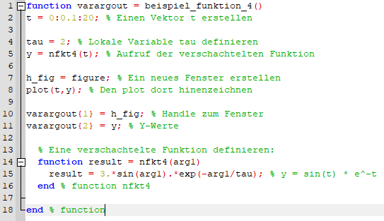
We can change the previous example slightly and move the local function into the example function. Since the function nfkt4 has then access to the variable tau of the function, we no longer need to pass the variables as arguments.

function varargout = example_function_4()
t = 0:0.1:20; % create vector t

tau = 2; % define local variable tau
y = nfkt4(t); % call the nested function

h_fig = figure; % create a new figure window
plot(t,y); % plot y over t

varargout{1} = h_fig; % handle to the figure window
varargout{2} = y; % y values

  % define a nested function:
  function result = nfkt4(arg1)
    result = 3.*sin(arg1).*exp(-arg1/tau); % y = sin(t) * e^-t 
  end % function nfkt4

end % function

The indentation of the function has no effect, also the comment % function after the end statement is optional – this only improves the readability.

Many Matlab programs are programmed in such a scheme, for example user interfaces created via “GUIDE”. A clear advantage is that such a program, when encapsulated in a function, can call any number of nested sub-functions and can be called from any location, since global variables are not required.

For beginners, the necessity of debugging is disadvantageous: You only see the local variables when you set a breakpoint in the function. This is actually quite normal when programming, but with Matlab, there is no need to deal with the techniques at the beginning.